Fast Nonlinear Buckling Solver
Benchmarking Awatif Against Abaqus
1Introduction
Slender and lightweight structures are governed by their nonlinear response: large displacements and second-order effects decide whether the structure stands. This is precisely the regime in which conventional analysis is slowest and least reliable, so the check that matters most is the one engineers run last, or not at all.
The bottleneck is not the physics but the route taken to it. Conventional FEM walks to the answer: apply a fraction of the load, iterate to equilibrium with Newton's method, repeat. Near a critical point the tangent stiffness becomes ill-conditioned, increments are cut and retried, and the iteration count grows without the solution advancing. Almost all of the cost is spent traversing the load path, not resolving the final state.
Awatif removes the path. Its nonlinear solver does not step the load on and iterate its way forward; it resolves the equilibrium state directly, and it stays stable through the critical point that forces a conventional solver to cut increments and retry. Members are represented with cubic shape functions, so the bending response is captured exactly within each element.
This paper tests that claim against Abaqus on three buckling-sensitive frame problems, run with identical geometry, sections, material, and mesh. Awatif reproduces the Abaqus displacements to within 1.00% while reducing the equilibrium iterations needed to reach them by up to four orders of magnitude.
2Benchmark Cases
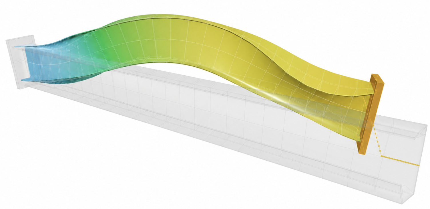
The three cases are chosen to cover the situations that punish an incremental solver. The cantilever column and the 3D portal frame are force-controlled, so the load path runs toward the critical point with no external control to stabilize it. The clamped-clamped IPE 300 column is displacement-controlled and carries a small weak-axis rest-curvature imperfection, so it passes through a genuine bifurcation into post-buckling and then unloads.
All three are modeled with frame elements, and both solvers receive the same model: the same geometry, sections, material, boundary conditions, and the same mesh of 10 to 20 segments per member. Awatif represents bending within each segment with a cubic shape function, which is the exact solution of the linear bending problem, so at these mesh densities the discretization is converged on both sides. Any difference that follows is attributable to the solver, not to the element or the mesh.
3Accuracy
Speed is only meaningful if the answer is the same, so accuracy is established first. For the cantilever column and portal frame, the compared value is the global X displacement at the loaded point. For the clamped-clamped IPE 300 column, it is the maximum global Z displacement near mid-span after buckling — the quantity that only exists because the member buckled, and therefore the sharpest test of whether both solvers found the same branch.
| Case | Compared displacement | Abaqus | Awatif | Difference |
|---|---|---|---|---|
| 1. Cantilever column | Global X at loaded point | 1.950 m | 1.929 m | 1.00% |
| 2. Portal frame | Global X at loaded point | 0.379 m | 0.382 m | 0.50% |
| 3. Clamped-clamped IPE 300 column | Maximum global Z near mid-span | 0.394 m | 0.393 m | 0.00% |
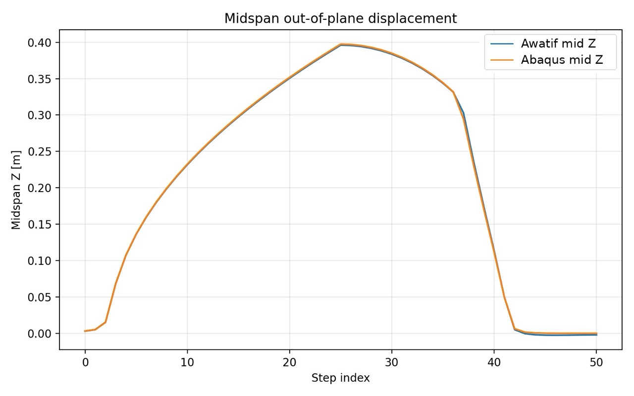
Endpoint agreement alone can be coincidental, so Figure 3 compares the entire mid-span out-of-plane history for the IPE 300 column. The two curves track each other throughout: the onset and growth of the weak-axis buckling displacement, the peak response, and the unloading-like reduction during the lateral displacement phase. Awatif does not merely arrive at the same final state — it follows the same physical response to get there, without stepping along the load path to do so.
4Performance
With accuracy established, performance is measured by the two quantities each solver reports about its own work: the equilibrium iterations required to reach the converged state, and the final residual error confirming that the state satisfies the convergence tolerance. Counting iterations rather than wall-clock time keeps the comparison independent of hardware, licensing, and process count, and isolates the behavior of the solver itself.
| Case | Abaqus iterations | Awatif iterations | Iteration speedup | Abaqus final error | Awatif final error |
|---|---|---|---|---|---|
| Cantilever column | 257,194 | 5 | 51,438.8× | 1.04 × 10⁻⁵ | 4.54 × 10⁻⁶ |
| Portal frame | 294,741 | 7 | 42,105.9× | 1.48 × 10⁻⁴ | 1.25 × 10⁻⁶ |
| IPE 300 column | 5,669 | 60 | 94.5× | 1.92 × 10⁻⁴ | 6.75 × 10⁻⁴ |
Iteration counts are each solver's own equilibrium iterations over the full analysis. A single iteration does not cost the same in both solvers, so the ratio measures how much path-following work was required rather than a literal wall-clock factor.
The pattern across the three cases tracks the difficulty of the load path. Both force-controlled cases drive the structure toward a critical point with no external control, which is where an incremental solver cuts and retries increments; both exceed a quarter of a million iterations in Abaqus and converge in fewer than ten in Awatif. The IPE 300 column is displacement-controlled, so the imposed displacement stabilizes the path and Abaqus never stalls in the same way — and it is exactly there that the gap narrows to 94.5×. The harder the load path, the larger the advantage, because the advantage comes from not having to trace it.
Fewer iterations does not mean a looser answer. On both force-controlled cases Awatif converges to a tighter final residual than Abaqus, by two orders of magnitude on the portal frame. On the IPE 300 column it settles at 6.75 × 10⁻⁴ against Abaqus's 1.92 × 10⁻⁴, the one case where its residual is the looser of the two, and the displacement comparison in Section 3 shows the difference to be immaterial.
5Conclusion
On the same models and the same meshes, Awatif reproduced the Abaqus response to within 1.00% on every benchmark, matched the full post-buckling history of the IPE 300 column, and reached those results with up to four orders of magnitude fewer equilibrium iterations. The two force-controlled cases, the ones a conventional solver finds hardest, showed the largest gains; the stabilized displacement-controlled case still improved by 94.5×.
The results support a single explanation. Conventional analysis is expensive because it walks the load path, and it is fragile for the same reason. Resolving equilibrium directly removes that cost without giving up the answer.
The scope here is deliberate: elastic frame elements, three benchmark cases, geometric nonlinearity only. The formulation is not restricted to them. The same framework is being extended to shell elements and to material nonlinearity, and the goal is a nonlinear check fast enough to run inside the design loop rather than after it.